Forecasting is the process of using existing data to predict future outcomes. This data includes past data, a.k.a. “historical data,” along with any additional, context-specific variables, a.k.a. “dynamic factors.”
Businesses can use forecasting to predict figures such as future sales or estimated foot traffic. Common applications include revenue projection, demand forecasting, and inventory optimization, to name a few.
Our software has the capacity to support forecasting across multiple locations, products, and scenarios. It also continually updates its results according to any changes in data or goals. Therefore, all predictions are based on the latest data available.
Data Preparation
The first step is to collect your data. Generally, the more data you have and the more detailed that data, the greater the accuracy of your predictions. More specifically, here are the key data categories to have for two common industries:
|
Consumer Retail |
Manufacturing |
minimum 2-5 yrs. of data recommended |
minimum 2-3 yrs. of data recommended |
To illustrate, take for example the following data set—it shows a bottled water company’s sales history, along with other key information such as product description, bottle size, price, etc.
| item id# | store# | date | quantity | category# | promotions | price | description | channel | size |
| 1 | 0 | 10/12/16 | 5 | 1 | none | 210 | sparkling water | W-Mart | 100ml |
| … | … | … | … | … | … | … | … | … | … |
| 2 | 1 | 9/24/17 | 1 | 1 | 50% off | 210 | sparkling water | Whole Goods | 1 L |
Platform Parameter Selection
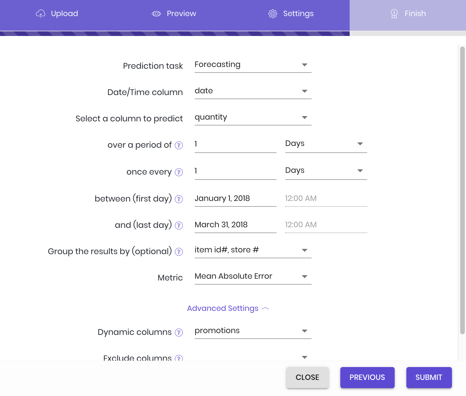
After uploading your data set, select “Forecasting” as your prediction task. The following menu will then appear, where you input your settings:

- Date/Time column: Choose the column in your data set that lists the date values. Note: while in our example that column is conveniently labeled “date,” that may not be the case for all data sets.
- Select column to predict: Choose the column in the data set that you want predictions for. Our example company wants predictions on how many items will sell in the upcoming months, and so chooses the “quantity” column that lists the number of each item sold.
- over a period of: Next, select the measure of time that you want the prediction to use. In the example, the company wants their total sales predictions measured by the day; the corresponding input is 1 day. Total sales by the week would be 1 week, and so on.
- once every: Select the regularity of the forecasts—in other words, the amount of time between each forecast start. To avoid overlap, this value will default to the “over a period of” input, but can be changed according to the situation. In our example, the value defaults to 1 day.
- between (first day): The start date of the stretch of time you want predictions for. The example company wants predictions from the start of January to the end of March, and sets January 1st as the first day.
- and (last day): The end date of the stretch of time you want predictions for. The example company wants predictions from the start of January to the end of March, and sets March 31st as the last day.
- Group results by: This setting is optional—feel free to leave it blank. Simply put, it allows you to select a particular level of granularity. In the example, the company decides that they don’t want just the total number of items sold—they also want to see how many of each item will sell in each store. So, they input the columns that list product code (item id#) and distribution center (store#).
- Metric: Simply put, a metric is a mathematical formula that measures the accuracy of the forecasted values. Each task has its own selection of metrics; with forecasting, the default tends to be Mean Absolute Error, a metric less sensitive to statistical outliers.
See available metrics
- Mean absolute error (MAE): \(\frac{1}{n}\sum_{i=1}^{n}|y_i-\hat{y}_i|\)
- Root mean square error (RMSE): \(\sqrt{\frac{1}{n}\sum_{i=1}^{n}(y_i-\hat{y}_i)^2}\)
- Mean absolute percentage error (MAPE): \(\frac{1}{n}\sum_{i=1}^{n}\frac{|y_i-\hat{y}_i}{y_i}\)
- Volume weighted mean absolute percentage error: \(\frac{\sum_{i=1}^{n}|y_i-\hat{y}_i|}{\sum_{i=1}^{n}|y_i|}\)
- Volume weighted forecasting accuracy: \(\sum_{i=1}^{n}\frac{y_i*\frac{min(y_i, \hat{y}_i)}{max(y_i, \hat{y}_i)}}{\sum_{i=1}^{n}y_i}\)
Advanced Settings
These settings are optional—if they hold no interest, feel free to leave them blank.
- Dynamic columns: If there are any dynamic factor columns you want to flag for future forecasts, you may list them here. In short, dynamic factors are situational, context-specific variables that shift based on the scenario—e.g., special promotions, marketing strategies, holidays, and so on. Please note that you cannot add to this list retroactively—any columns you want to test for must be listed at time of initial setup. For example, the water company plans to do future forecasts that test out different promotions, and lists the “promotions” column accordingly. For information on how to prepare dynamic factor data and generate new forecast results, see Preparation of Test Data with Dynamic Factors.
- Exclude columns: If there are any columns that you want the platform to ignore during model training, you may list them here.
General Tips
- Try to avoid long time intervals—e.g., multiple years—as predictions are likely to be less accurate. We recommend monthly or quarterly forecasts if working with around three years’ worth of historical data.
- If there are negative sales numbers in the sales data—a customer returning a purchase, for example—remove those figures whenever possible.
- Make sure the time format is correct. While our platform can automatically account for common date formats (e.g., “YYYY-MM-DD”, “YYYY/MM/DD”, “DD/MM/YY”, etc.), we strongly recommend that users ensure the time format is consistent in order to avoid inaccuracy.
- For weekly data, use a fixed weekday as the start of every week to avoid making the model process different week formats. For example: if the week starts on Mondays, that should be consistent throughout the data set (as opposed to Friday or Saturday, etc.).
- The platform forecast automatically includes the last date of the forecast range, so you don’t have to consider the actual end date of the forecast. For example: if forecasting monthly sales for September 2018, the forecast end can be listed as 09/01/2018.
- The platform currently supports one date/time column only. If date and time data are in two separate columns, merge them into one column and resubmit. For example: one date column listing “2017-01-01” and one time column listing “12:00:00” must be merged into one column listing “2017-01-01 12:00:00”.
Preparation of Test Data with Dynamic Factors
To generate new dynamic factor forecasts, first upload a new data set that includes the following columns:
A) the group column(s) set during model set-up (listed under “Group results by:”)
B) a date/time column, and
C) the dynamic factor column(s)
You need to provide dynamic factor information for each item that you want predictions for—starting with the end date in the training data set, and ending with the end date of the new forecast. (We start with the training set end date to account for any new modifying factors introduced in the time period between the training set end date and the start date of the new forecast.) If there are missing values, the platform will approximate them based on prior data.
For instance, our example company wants to predict the daily sales of a specific product (item id# 1) at a specific retail location (store# 0) during the same time period of January to March, but without the promotion that had been applied to it (from “50% off” to “none”). They create the following data set:
Table 2: Test Data with Dynamic Factors
| item id# | store# | date | promotions | category# |
| 1 | 0 | 09/24/17 | none | 1 |
| 1 | 0 | 09/25/17 | none | 1 |
| … | … | … | … | … |
| 1 | 0 | 03/31/2018 | none | 1 |
To generate the forecast, enter a command in the chat box in the following format: “@eva, apply model [#model_id/#task_id] to data [#data_id].” (You can find these values by hovering over each file in the AI Tasks and Data tabs, clicking the icon appearing to the far right, then “Copy ID.”) Our helpful robot assistant Eva will then provide you with a download link to your new predictions.
Dynamic Factor FAQ
- Can I predict retroactively—in other words, figure out what my values could have been during the training data time period?
- No, we don’t support that function for the time being. You can set prediction time intervals only after the end of the training data time period. For example, with training data ending at 12/31/2017, you can only make predictions from 01/01/2018 onward.
- Can I predict values beyond the forecast range that I initially selected?
- No. At this time, the platform does not support updating that initial data. You can only generate forecasts within the originally-set time interval. For example, if the set interval was 02/01/2018 to 03/31/2018, the test range could be from that time period only. You wouldn’t be able to predict sales after 03/31/2018. You can, however, create a new model with a different forecast range.
- Can I predict combinations of dynamic factors that did not exist in the training data?
- Yes, you can! For example, a new product wouldn’t have historical sales records, but you could make predictions based on other characteristics of the product, provide the appropriate dynamic factor information, and make a prediction from there.
User Case
This case is based on a Kaggle.com competition in which participants generated sales forecasts for Rossmann, a European drugstore chain. The original data is available for download on the competition page: https://www.kaggle.com/c/rossmann-store-sales
Alternatively, you can download our pre-prepared sample data: https://s3-us-west-2.amazonaws.com/oneclick.ai-demo-date/rossmann_store_sales.zip
The data includes daily sales info for 1,115 stores, from January 1, 2013 to July 31, 2015. It also contains columns recording promotional information (1/0 as promotion/no promotion), whether or not the store was open that day (1/0 as open/closed), holiday information for both national holidays and school holidays (1/0 as holiday/no holiday), along with store category information (a/b/c/d as the different categories).
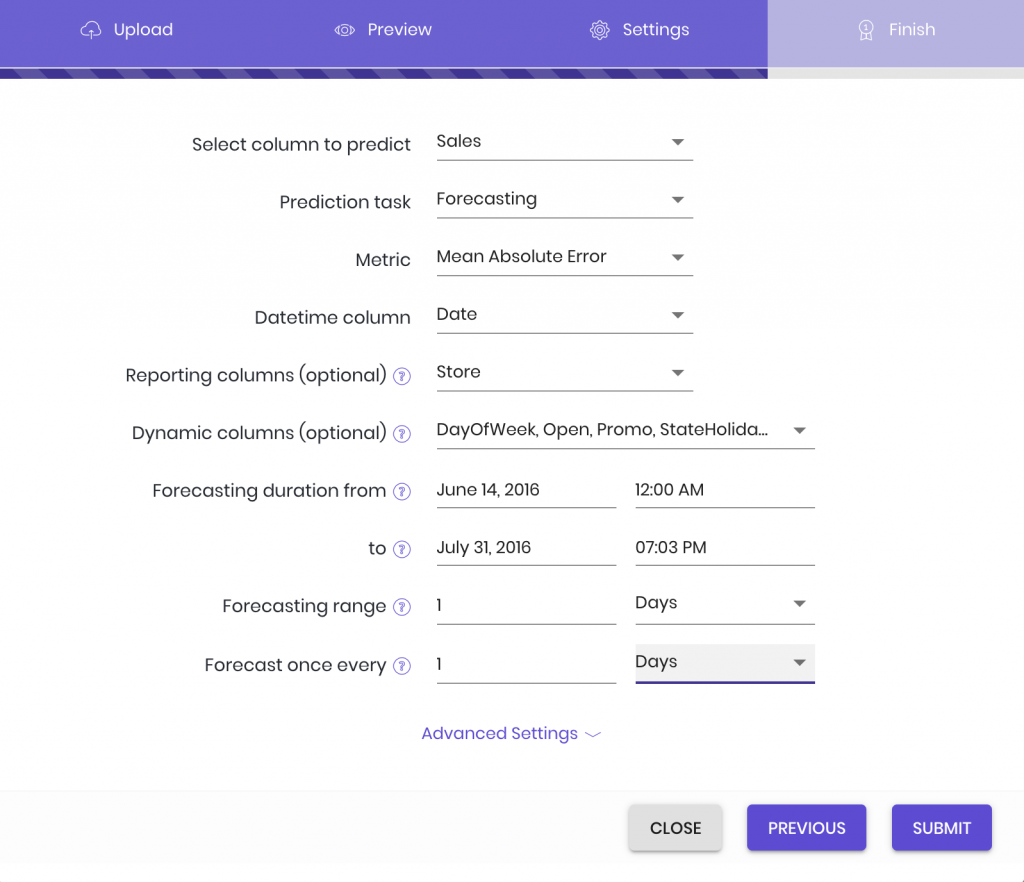
From this original data set, we selected stores 1-15 for our data pool. We then chose all the data before June 13, 2015 for our training data set, and set June 14, 2015—July 31, 2015 as our desired range for sales predictions. (We’ll be comparing our predictions to how much the stores actually sold.) After uploading the training data to the platform, we set our parameters as follows:
Rossmann Store Sales Forecasting Settings


After the model training, we uploaded the test interval’s dynamic factor data, and entered the appropriate command in the chat box. This summons our robot friend Eva to present us with our predictions:


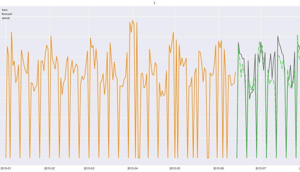
Here is a visualization of the forecast results compared to the stores’ actual sales:
Actual Sales Figures vs. Predicted Sales Figures


Dynamic Factor Tuning
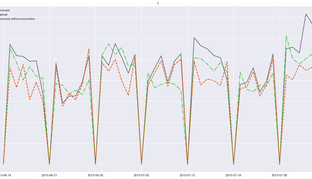
We can alter dynamic factors to see the effects of various scenarios and determine optimal business strategies. In this example, if we want to know which promotion plans are most effective, we can try out new dynamic factor forecasts with different promotion data sets. For example, in the original data set, promotions happen every other week. If we try out a prediction with no promotions at all, the results are as follows:
Bi-Weekly Forecasts: Promotion vs. No Promotion


We can see that for every other week, no promotions means less revenue—so, the business knows when best to have those promos!
Related Readings
Applications of forecasting:
For a detailed case study using forecasting:


